[1]:

import matplotlib.pyplot as plt
from vangja.datasets.loaders import load_kaggle_temperature, load_smart_home_readings

Our goal is to predict the daily energy consumption of smart home appliances based. Our train data contains only 3 months of energy consumption readings, which is not enough to train a robust model. To overcome this challenge, we will leverage external data sources, specifically the daily maximum temperature readings for the city of Boston, to enhance our model’s performance. We will use the temperature data to train a model that can capture yearly seasonality patters, which will be transferred to the energy consumption model to improve its predictions.

1. Data preparation and loading#

We start by loading the necessary datasets for our case study. We will be working with two datasets: one containing daily energy consumption readings from a smart home, and another containing daily maximum temperature readings for the city of Boston.

First, we load the temperature data for Boston from the Kaggle dataset. We specify the city, the date range, and the frequency of the data we want to load. We use the date range from January 1, 2014, to March 31, 2016, to ensure we have at least two full years of data for our analysis and to ensure there is no data leakage i.e. the temperature data does not include future information.

[ ]:

temp_df = load_kaggle_temperature(
    city="Boston", start_date="2014-01-01", end_date="2016-03-31", freq="D"
)
temp_df

	ds	y
0	2014-01-01	-5.765000
1	2014-01-02	-6.108125
2	2014-01-03	-14.362083
3	2014-01-04	-12.607497
4	2014-01-05	-2.569375
...	...	...
816	2016-03-27	2.793056
817	2016-03-28	4.026540
818	2016-03-29	7.176683
819	2016-03-30	5.664472
820	2016-03-31	9.879861

821 rows × 2 columns

[3]:

def plot_both_dfs(df1, df2, title1="Series 1", title2="Series 2"):
    # Visualize both time series
    fig, axes = plt.subplots(2, 1, figsize=(14, 8), sharex=False)

    # Temperature
    axes[0].plot(df1["ds"], df1["y"], "C0-", linewidth=0.5, alpha=0.7)
    axes[0].set_title(title1)
    axes[0].set_ylabel("Temperature (°C)")
    axes[0].grid(True, alpha=0.3)

    # Sales
    axes[1].plot(df2["ds"], df2["y"], "C1-", linewidth=0.5, alpha=0.7)
    axes[1].set_title(title2)
    axes[1].set_ylabel("Number of Sales")
    axes[1].set_xlabel("Date")
    axes[1].grid(True, alpha=0.3)

    plt.tight_layout()
    plt.show()

We then load the energy consumption data from the smart home dataset. We specify the columns we are interested in, which include the energy consumption readings for Furnace 1, Furnace 2, Fridge, and Wine cellar. We also specify the frequency of the data as daily.

[4]:

smart_home_df = load_smart_home_readings(
    column=["Furnace 1 [kW]", "Furnace 2 [kW]", "Fridge [kW]", "Wine cellar [kW]"],
    freq="D",
)
smart_home_df

[4]:

	ds	y	series
0	2016-01-01	0.083106	Fridge [kW]
1	2016-01-02	0.051980	Fridge [kW]
2	2016-01-03	0.063992	Fridge [kW]
3	2016-01-04	0.049317	Fridge [kW]
4	2016-01-05	0.055650	Fridge [kW]
...	...	...	...
1399	2016-12-12	0.028141	Wine cellar [kW]
1400	2016-12-13	0.021090	Wine cellar [kW]
1401	2016-12-14	0.027129	Wine cellar [kW]
1402	2016-12-15	0.018033	Wine cellar [kW]
1403	2016-12-16	0.085299	Wine cellar [kW]

1404 rows × 3 columns

1.1 Data visualization#

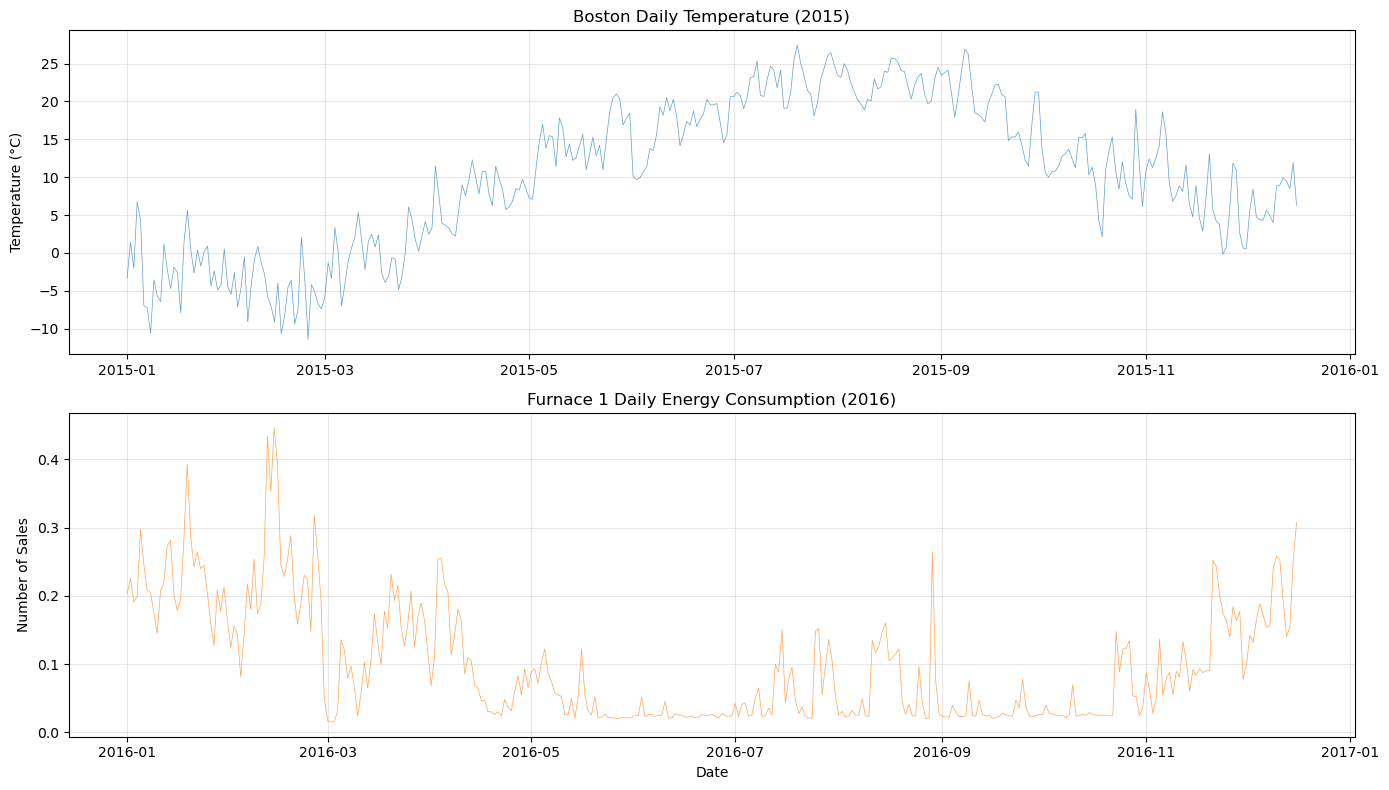
Let’s plot the temperature and energy consumption data to visualize the patterns and relationships between them.

[5]:

plot_both_dfs(
    temp_df[(temp_df["ds"] >= "2015-01-01") & (temp_df["ds"] <= "2015-12-16")],
    smart_home_df[smart_home_df["series"] == "Furnace 1 [kW]"],
    title1="Boston Daily Temperature (2015)",
    title2="Furnace 1 Daily Energy Consumption (2016)",
)

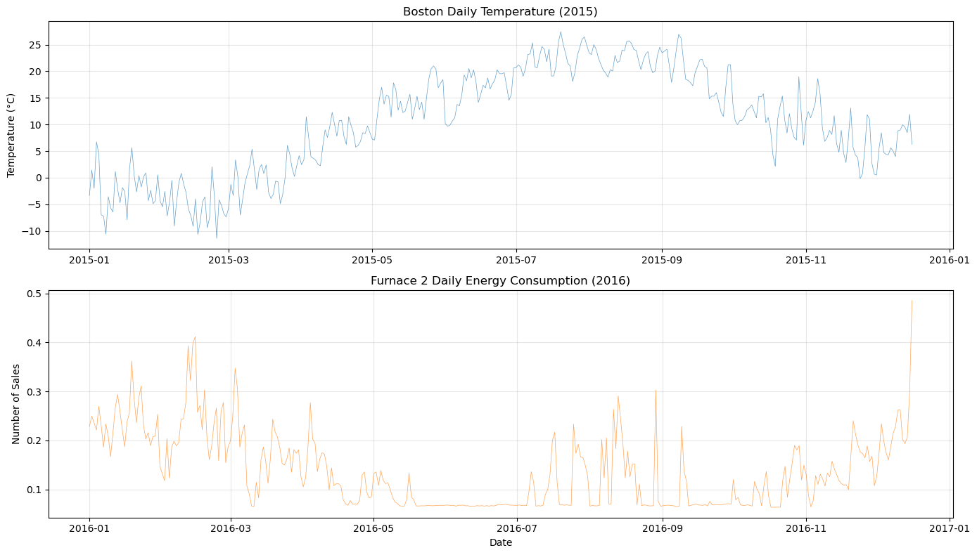
../_images/notebooks_01_case_study_smart_home_7_0.png

[6]:

plot_both_dfs(
    temp_df[(temp_df["ds"] >= "2015-01-01") & (temp_df["ds"] <= "2015-12-16")],
    smart_home_df[smart_home_df["series"] == "Furnace 2 [kW]"],
    title1="Boston Daily Temperature (2015)",
    title2="Furnace 2 Daily Energy Consumption (2016)",
)

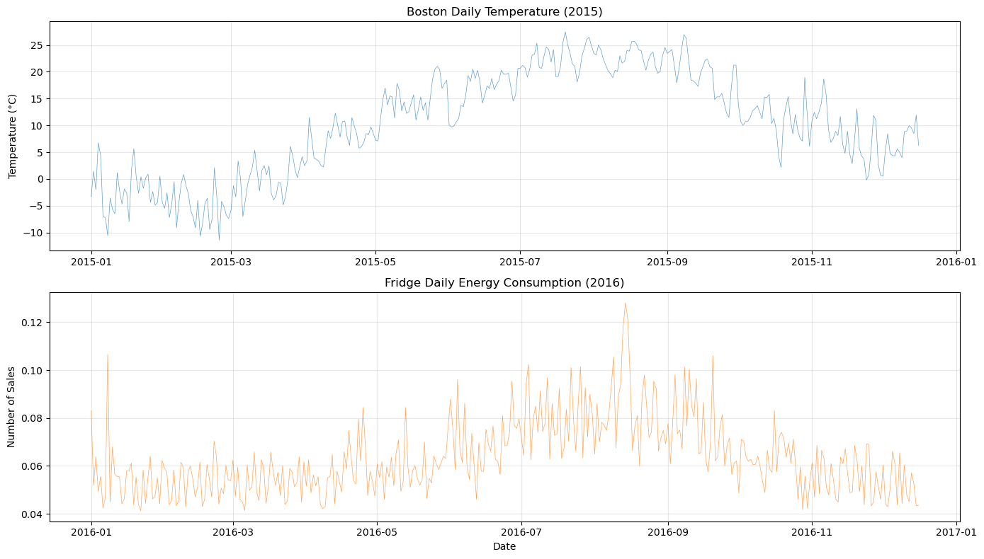
../_images/notebooks_01_case_study_smart_home_8_0.png

[7]:

plot_both_dfs(
    temp_df[(temp_df["ds"] >= "2015-01-01") & (temp_df["ds"] <= "2015-12-16")],
    smart_home_df[smart_home_df["series"] == "Fridge [kW]"],
    title1="Boston Daily Temperature (2015)",
    title2="Fridge Daily Energy Consumption (2016)",
)

../_images/notebooks_01_case_study_smart_home_9_0.png

[8]:

plot_both_dfs(
    temp_df[(temp_df["ds"] >= "2015-01-01") & (temp_df["ds"] <= "2015-12-16")],
    smart_home_df[smart_home_df["series"] == "Wine cellar [kW]"],
    title1="Boston Daily Temperature (2015)",
    title2="Wine Cellar Daily Energy Consumption (2016)",
)

../_images/notebooks_01_case_study_smart_home_10_0.png

2. Predictive checks and model training - temperature model#

[9]:

from vangja import FlatTrend, FourierSeasonality
from vangja.utils import plot_prior_predictive, prior_predictive_coverage

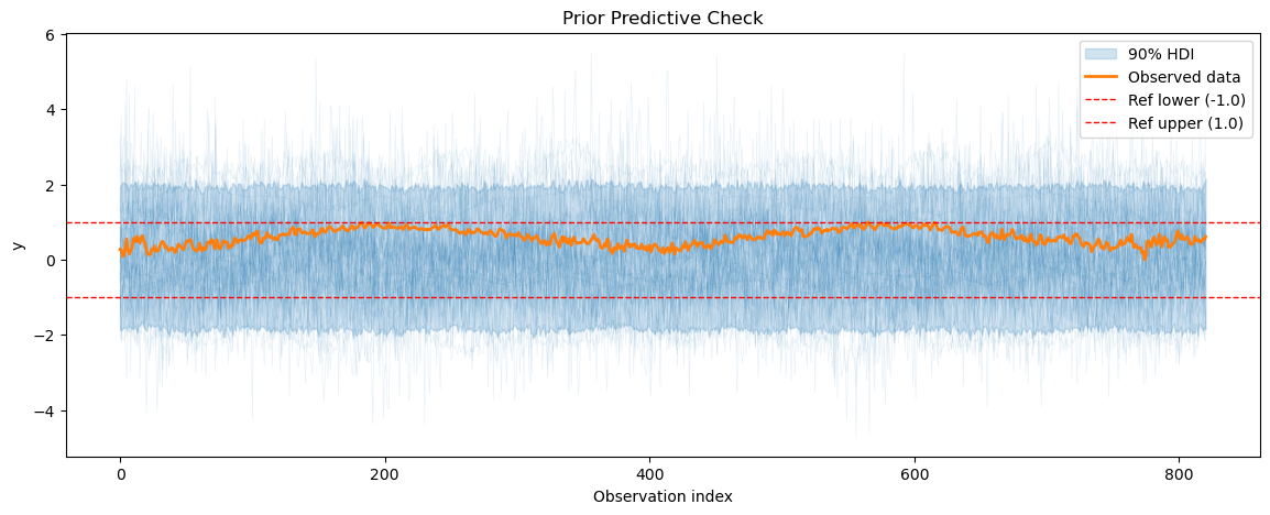
def create_temp_model():
    return FlatTrend(intercept_sd=1) + FourierSeasonality(
        period=365, series_order=5, beta_sd=0.1
    )

temp_model = create_temp_model()
temp_model.fit(temp_df, scaler="minmax", method="mapx")
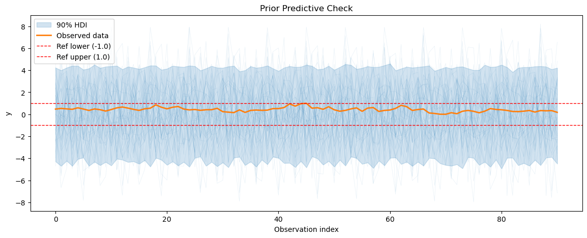
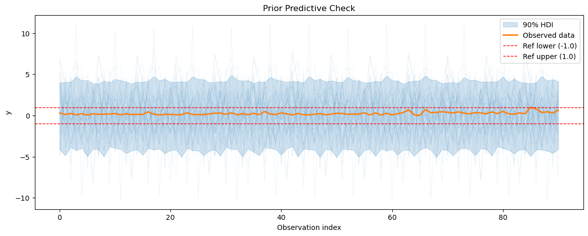
temp_prior_pred = temp_model.sample_prior_predictive()
plot_prior_predictive(
    temp_prior_pred, data=temp_model.data, show_hdi=True, show_ref_lines=True
)
print(f"Prior predictive coverage: {prior_predictive_coverage(temp_prior_pred)}")

WARNING:2026-03-14 20:49:09,504:jax._src.xla_bridge:876: An NVIDIA GPU may be present on this machine, but a CUDA-enabled jaxlib is not installed. Falling back to cpu.

Sampling: [fs_0 - beta(p=365,n=5), ft_0 - intercept, obs, sigma]

Prior predictive coverage: 0.9137904993909866

../_images/notebooks_01_case_study_smart_home_12_5.png

[10]:

temp_model = create_temp_model()
temp_model.fit(temp_df, scaler="minmax", method="nuts")

Multiprocess sampling (4 chains in 4 jobs)
NUTS: [ft_0 - intercept, fs_0 - beta(p=365,n=5), sigma]
/home/jovan/miniconda3/envs/vangja20/lib/python3.13/multiprocessing/popen_fork.py:67: RuntimeWarning: os.fork() was called. os.fork() is incompatible with multithreaded code, and JAX is multithreaded, so this will likely lead to a deadlock.
  self.pid = os.fork()

/home/jovan/miniconda3/envs/vangja20/lib/python3.13/multiprocessing/popen_fork.py:67: RuntimeWarning: os.fork() was called. os.fork() is incompatible with multithreaded code, and JAX is multithreaded, so this will likely lead to a deadlock.
  self.pid = os.fork()

Sampling 4 chains for 1_000 tune and 1_000 draw iterations (4_000 + 4_000 draws total) took 5 seconds.

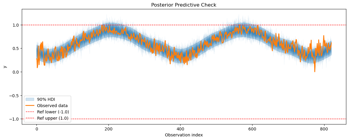
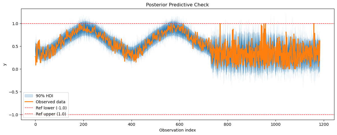
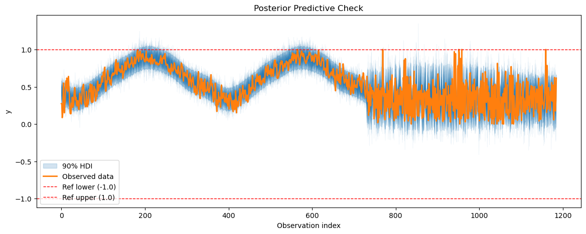
[11]:

from vangja.utils import plot_posterior_predictive


temp_posterior_pred = temp_model.sample_posterior_predictive()
plot_posterior_predictive(temp_posterior_pred, temp_model.data, show_hdi=True, show_ref_lines=True)

Sampling: [obs]

[11]:

<Axes: title={'center': 'Posterior Predictive Check'}, xlabel='Observation index', ylabel='y'>

../_images/notebooks_01_case_study_smart_home_14_4.png

3. Predictive checks and model training - energy consumption model#

[38]:

import pandas as pd

from vangja.components.uniform_constant import UniformConstant
from vangja.utils import metrics

smh_train_df = smart_home_df[smart_home_df["ds"] < "2016-04-01"]
smh_test_df = smart_home_df[smart_home_df["ds"] >= "2016-04-01"]

test_temp_df = load_kaggle_temperature(
    city="Boston", start_date="2016-04-01", end_date="2016-12-16", freq="D"
)
temp_df["series"] = "Temperature"
test_temp_df["series"] = "Temperature"

train_df = pd.concat([smh_train_df, temp_df], ignore_index=True)
test_df = pd.concat([smh_test_df, test_temp_df], ignore_index=True)

smart_home_model = (
    FlatTrend(intercept_sd=1, pool_type="individual")
    + UniformConstant(lower=-1, upper=1, pool_type="partial")
    * FourierSeasonality(
        period=365,
        series_order=5,
        beta_sd=1,
        tune_method="parametric",
        pool_type="partial",
        loss_factor_for_tune=0,
    )
    + FourierSeasonality(period=7, series_order=3, beta_sd=1, pool_type="partial")
)
smart_home_model.fit(
    train_df,
    scaler="minmax",
    method="nuts",
    scale_mode="individual",
    sigma_pool_type="individual",
    t_scale_params=temp_model.t_scale_params,
    idata=temp_model.trace,
)
smart_home_prior_pred = smart_home_model.sample_prior_predictive()
future = smart_home_model.predict_uncertainty(horizon=365)
smart_home_model_metrics = metrics(test_df, future, pool_type="partial")
smart_home_model_metrics

Multiprocess sampling (4 chains in 4 jobs)
NUTS: [ft_0 - intercept, uc_0 - c_shared, uc_0 - c_sigma, uc_0 - c_offset, fs_0 - beta_shared, fs_0 - beta_sigma(p=365,n=5), fs_0 - beta_z_offset(p=365,n=5), fs_1 - beta_shared, fs_1 - beta_sigma(p=7,n=3), fs_1 - beta_z_offset(p=7,n=3), sigma]
/home/jovan/miniconda3/envs/vangja20/lib/python3.13/multiprocessing/popen_fork.py:67: RuntimeWarning: os.fork() was called. os.fork() is incompatible with multithreaded code, and JAX is multithreaded, so this will likely lead to a deadlock.
  self.pid = os.fork()

/home/jovan/miniconda3/envs/vangja20/lib/python3.13/multiprocessing/popen_fork.py:67: RuntimeWarning: os.fork() was called. os.fork() is incompatible with multithreaded code, and JAX is multithreaded, so this will likely lead to a deadlock.
  self.pid = os.fork()

Sampling 4 chains for 1_000 tune and 1_000 draw iterations (4_000 + 4_000 draws total) took 608 seconds.
There were 5 divergences after tuning. Increase `target_accept` or reparameterize.
/home/jovan/repos/vangja/src/vangja/time_series.py:932: UserWarning: The effect of Potentials on other parameters is ignored during prior predictive sampling. This is likely to lead to invalid or biased predictive samples.
  return pm.sample_prior_predictive(samples=samples)
Sampling: [fs_0 - beta_shared, fs_0 - beta_sigma(p=365,n=5), fs_0 - beta_z_offset(p=365,n=5), fs_1 - beta_shared, fs_1 - beta_sigma(p=7,n=3), fs_1 - beta_z_offset(p=7,n=3), ft_0 - intercept, obs, sigma, uc_0 - c_offset, uc_0 - c_shared, uc_0 - c_sigma]
/home/jovan/repos/vangja/src/vangja/time_series.py:582: FutureWarning: The return type of `Dataset.dims` will be changed to return a set of dimension names in future, in order to be more consistent with `DataArray.dims`. To access a mapping from dimension names to lengths, please use `Dataset.sizes`.
  n_chains = posterior.dims["chain"]
/home/jovan/repos/vangja/src/vangja/time_series.py:583: FutureWarning: The return type of `Dataset.dims` will be changed to return a set of dimension names in future, in order to be more consistent with `DataArray.dims`. To access a mapping from dimension names to lengths, please use `Dataset.sizes`.
  n_draws = posterior.dims["draw"]

[38]:

	mse	rmse	mae	mape
Fridge [kW]	0.000251	0.015837	0.011638	0.160868
Furnace 1 [kW]	0.003236	0.056887	0.041898	0.822217
Furnace 2 [kW]	0.003512	0.059260	0.039558	0.348530
Temperature	11.556069	3.399422	2.646411	0.453586
Wine cellar [kW]	0.000799	0.028265	0.017561	0.312579

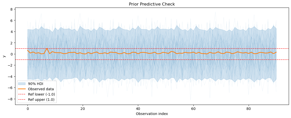
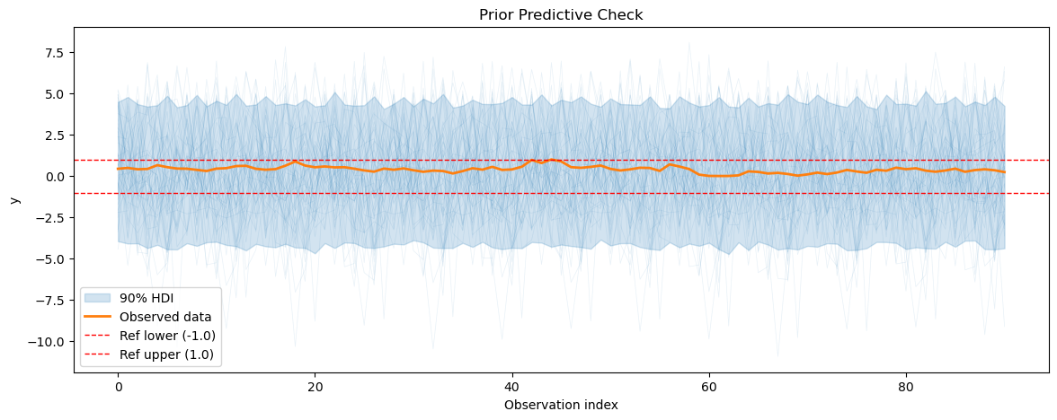
[39]:

for series_idx in range(smart_home_model.n_groups):
    plot_prior_predictive(
        smart_home_prior_pred,
        data=smart_home_model.data,
        series_idx=series_idx,
        group=smart_home_model.group,
        show_hdi=True,
        show_ref_lines=True,
    )
    print(
        f"Prior predictive coverage (series {series_idx}): {prior_predictive_coverage(smart_home_prior_pred, series_idx=series_idx, group=smart_home_model.group)}"
    )

Prior predictive coverage (series 0): 0.5512307692307692
Prior predictive coverage (series 1): 0.5612087912087912
Prior predictive coverage (series 2): 0.5507032967032967
Prior predictive coverage (series 3): 0.5497247259439708
Prior predictive coverage (series 4): 0.5580219780219781

../_images/notebooks_01_case_study_smart_home_17_1.png

../_images/notebooks_01_case_study_smart_home_17_2.png

../_images/notebooks_01_case_study_smart_home_17_3.png

../_images/notebooks_01_case_study_smart_home_17_4.png

../_images/notebooks_01_case_study_smart_home_17_5.png

[ ]:

smh_posterior_pred = smart_home_model.sample_posterior_predictive()
for series_idx in range(smart_home_model.n_groups):
    plot_posterior_predictive(
        smh_posterior_pred,
        data=smart_home_model.data,
        series_idx=series_idx,
        group=smart_home_model.group,
        show_hdi=True,
        show_ref_lines=True,
    )

/home/jovan/repos/vangja/src/vangja/time_series.py:968: UserWarning: The effect of Potentials on other parameters is ignored during posterior predictive sampling. This is likely to lead to invalid or biased predictive samples.
  return pm.sample_posterior_predictive(self.trace)
Sampling: [obs]

../_images/notebooks_01_case_study_smart_home_18_3.png

../_images/notebooks_01_case_study_smart_home_18_4.png

../_images/notebooks_01_case_study_smart_home_18_5.png

../_images/notebooks_01_case_study_smart_home_18_6.png

../_images/notebooks_01_case_study_smart_home_18_7.png

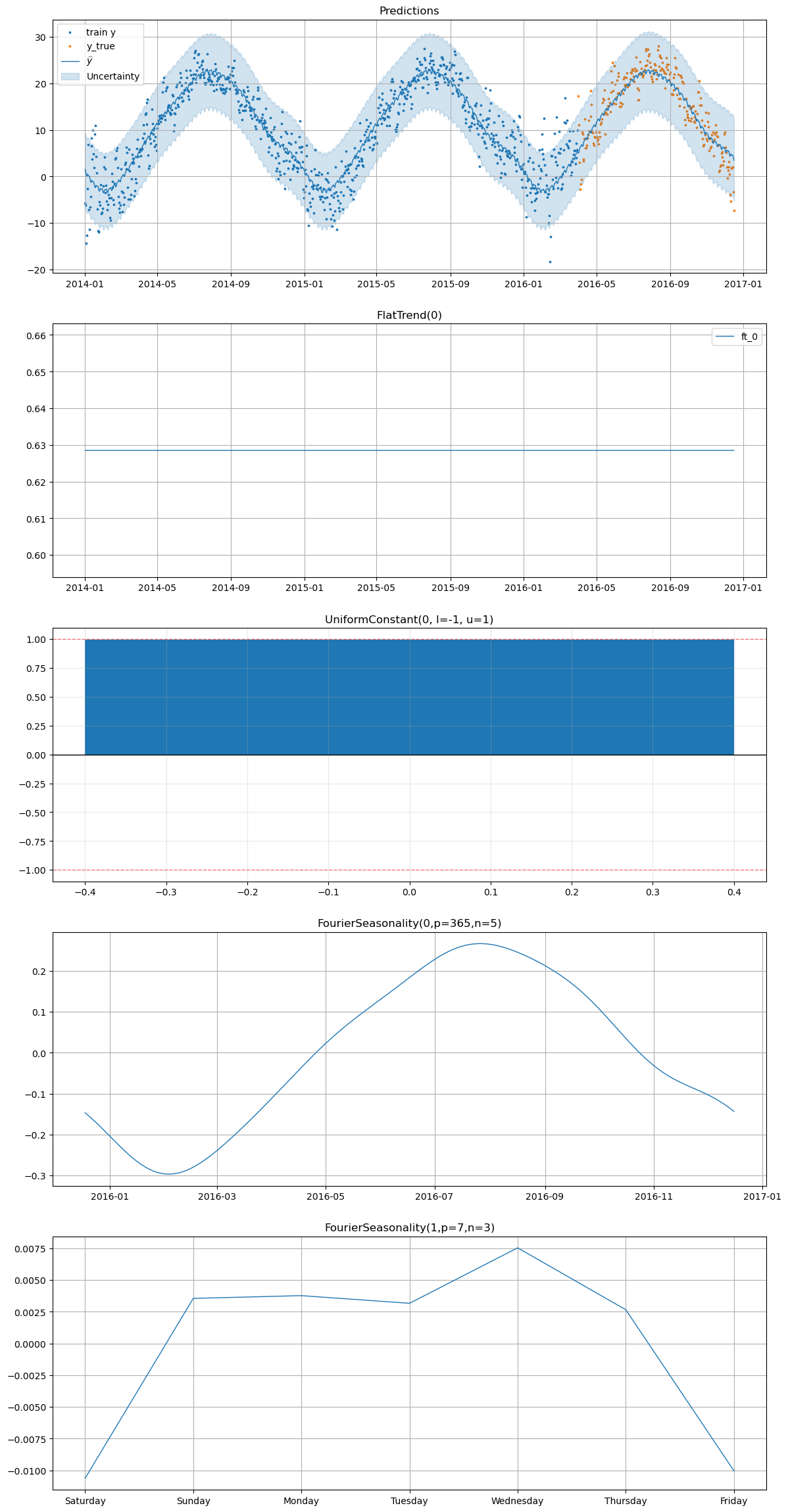
[37]:

smart_home_model.plot(
    future,
    series="Temperature",
    y_true=test_df[
        (test_df["series"] == "Temperature") & (test_df["ds"] >= "2016-04-01")
    ],
)

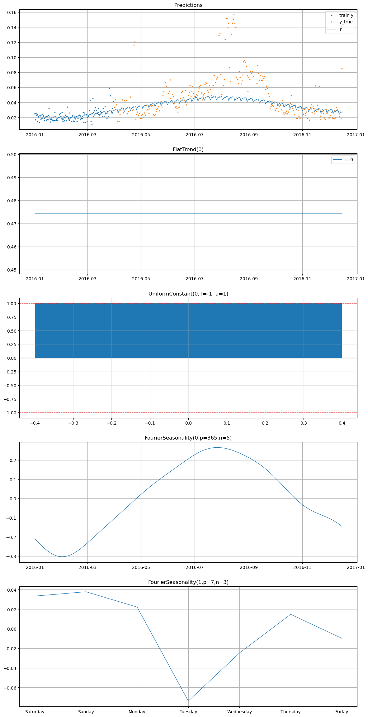
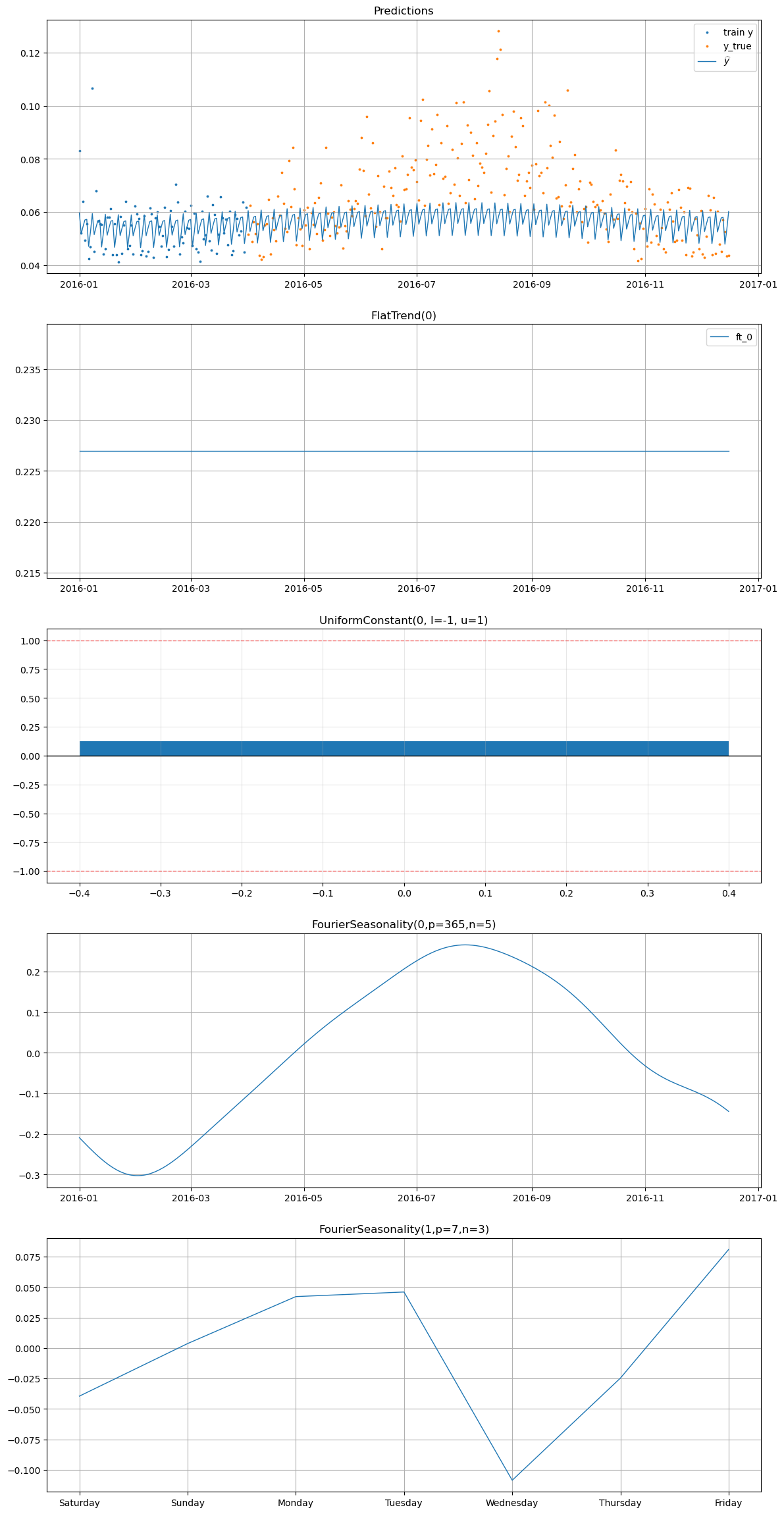
../_images/notebooks_01_case_study_smart_home_19_0.png

[36]:

smart_home_model.plot(
    future,
    series="Furnace 1 [kW]",
    y_true=smart_home_df[
        (smart_home_df["series"] == "Furnace 1 [kW]")
        & (smart_home_df["ds"] >= "2016-04-01")
    ],
)

../_images/notebooks_01_case_study_smart_home_20_0.png

[26]:

smart_home_model.plot(
    future,
    series="Furnace 2 [kW]",
    y_true=smart_home_df[
        (smart_home_df["series"] == "Furnace 2 [kW]")
        & (smart_home_df["ds"] >= "2016-04-01")
    ],
)

../_images/notebooks_01_case_study_smart_home_21_0.png

[23]:

smart_home_model.plot(
    future,
    series="Fridge [kW]",
    y_true=smart_home_df[
        (smart_home_df["series"] == "Fridge [kW]")
        & (smart_home_df["ds"] >= "2016-04-01")
    ],
)

../_images/notebooks_01_case_study_smart_home_22_0.png

[24]:

smart_home_model.plot(
    future,
    series="Wine cellar [kW]",
    y_true=smart_home_df[
        (smart_home_df["series"] == "Wine cellar [kW]")
        & (smart_home_df["ds"] >= "2016-04-01")
    ],
)

../_images/notebooks_01_case_study_smart_home_23_0.png

1. Data preparation and loading

Contents

1. Data preparation and loading#

1.1 Data visualization#

2. Predictive checks and model training - temperature model#

3. Predictive checks and model training - energy consumption model#